
I’ve written a tuning process with some additional explanations. You can download that document on the Testgear section of this site. It’s called “A Straightforward One Seat Tuning Process and Some Notes About Why it Works”. In it, I suggest a process that can be used in the installation bay for tuning cars that’s effective and efficient. It’s great for DIYers too. For some readers, this process may differ greatly from what you’ve been told by numerous enthusiasts, sound quality judges and other accomplished tuners. So, before we get started here, I’d like to explain why.
There’s a big difference between tuning cars as a profession and tuning cars as a hobby. For the hobbyist, the tuning is often the end rather than the means—the tuner likes to spend hours experimenting, listening and retuning. For the professional, these extra hours spent on listening and retuning eat into our ability to move on to the next car and our ability to satisfy the next customer.
First, my objective in all of the tech tips I write, whether those tips are on the Audiofrog web forum, on Facebook or in articles like this one, is to provide an appropriate balance between speed, predictability and performance. In the interest of speed and predictability, I favor objective processes—those that don’t require us to use our ears and make a thousand subjective analyses and an endless series of adjustments. There’s a place for subjective analysis, but that’s after all objective measures have been exhausted.
There’s a temptation among many of us to see the speedy and objective process as worse than the lengthy “artisan” process of tuning primarily by ear. This is a fallacious argument if the quality of the performance that the two processes provide is the same or even similar. Additional time invested isn’t always “additional performance”.
Here’s an example: every subwoofer box built for a round subwoofer needs a hole in the baffle that fits the subwoofer. What’s the appropriate tool? Most of us would immediately say it’s a router with a circle template or a circle cutting jig. For some, the answer is a CNC router. We don’t bash these processes as lacking the necessary opportunity to include our “art” or our skill in the process, even though cutting the circle freehand and with no line to follow using a jigsaw would better demonstrate our circle cutting skills.
What are the chances that we’d cut a circle with a jigsaw and no guide to follow as accurately as our CNC machine? Not good. Eventually, with a series of files and sandpaper, we might get close and after a much longer process, we could demonstrate that the outcomes are similar. What’s the difference? Cost. If we’re a pro charging the customer $30 to cut a round hole, then it behooves us to use the most efficient method that provides an appropriate outcome.
In our circle cutting example, the objective process is not only speedier, but it’s more accurate, too. Determining if the circle is correct is a simple matter—either the speaker fits or it doesn’t fit.
“Hey, there’s a difference. Sound is subjective but a circle isn’t!”
Yes, that’s true. Sound is somewhat subjective. Some customers prefer more bass. Some prefer less high frequency content. That doesn’t change what a stereo system and a stereo recording are designed to do. That design dictates what’s correct. The system is correct when the left and right frequency responses match and the signals arrive at the listener in phase. After we arrive at correct, then we can make some adjustments for personal preference.
When we are tuning cars, our objective tools and the information they display allow us to see easily how far from correct we are in each step of the process. Because of the way our brains work in processing what we hear, it’s helpful for us to use analysis methods that correlate well with what we hear. Some measurement processes are better than others.
We’re all probably familiar with the situation in which the RTA curve appears to be correct, but the car sounds terrible. In some cases, tuners use this as a reason to reject the tool, rather than to look deeper into the reason that what appears to be correct is not. The first question to ask in that situation is “does this measurement make sense” and the second is “what am I really measuring?” The RTA doesn’t lie, but it also doesn’t completely characterize the performance of the system. It shows us one aspect of performance.
Do tools exist that allow us to completely characterize the performance of the system? Sure. Do we all know how to use them? No. Is it necessary to completely characterize and correct everything? No.
Our next consideration should be “which deviations from correct are inaudible?” We don’t need to focus on those. If we don’t need to focus on them, then we don’t need to spend money and time analyzing them during a production tuning process. As a skills-building exercise to be conducted on our own time, learning those processes and how to use those tools may make us better able to identify problems and solutions, but those activities should be extracurricular. When we’ve improved those skills to the point at which we can deploy them to increase accuracy, predictability or efficiency, we should introduce them into our process.
The objective of this article is to clear up a few misunderstandings about what we measure, what it means and what’s sufficient based on audibility.
The first topic is frequency response measurements. Is a single microphone measurement sufficient or do we need to make multiple measurements and find an average? There’s no question among acousticians that the multiple-mic measurement technique better correlates with what we hear. That means that what we see on the graph looks more like what we experience, but by how much and what’s the basis for this process?
For car stereo systems optimized for one seat, we are primarily concerned about performance for the driver. We often think of this position as completely stationary. The driver looks forward at the road while he drives, right? Hmmm…maybe not. We move our heads all the time. We look to the left, we look to the right, we look up and down. Sometimes we do that unconsciously in order to localize sounds we hear. A spatial average measurement is meant to approximate these head movements and to eliminate a comb filter that we measure with a single mic but that we don’t hear with our ears in the same way.
In the frequency response measurement in figure 1, there are five measurements displayed. These measurements of the passenger’s side speaker system, including the sub, were made with the microphone in the driver’s seat. The microphone was placed in 5 positions in a 7” circle.
Figure 1.
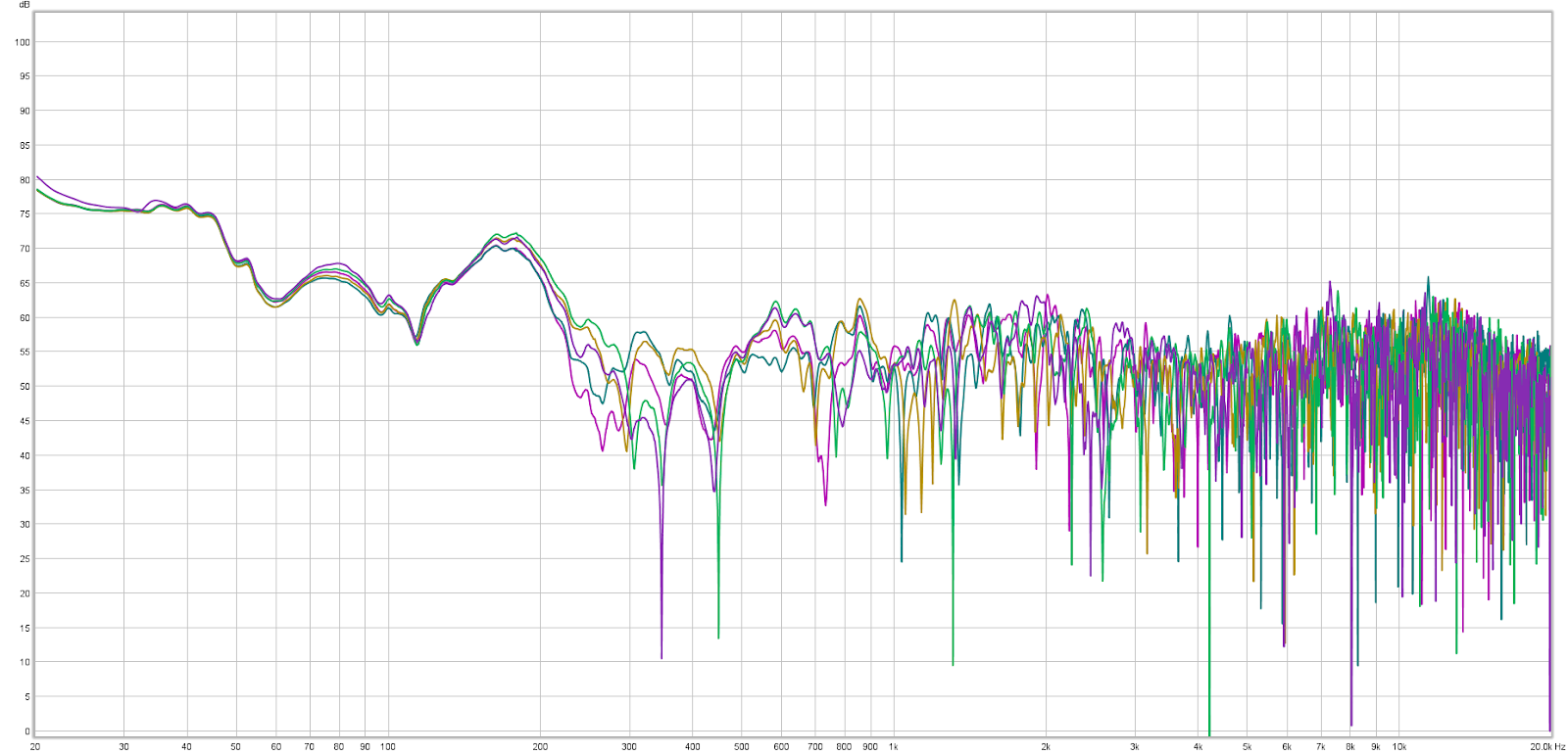
[Figure 1 caption: Unsmoothed measurements made in a 7” circle around the driver’s head position]
It’s pretty easy to see that there are two distinct regions and a transition region. Below 200Hz, the five measurements are very similar. No matter where we move our head (or the microphone), we hear the same thing. Above 1kHz, the measurements vary a lot. Moving the mic changes the frequency response by 25dB or more. Not only do the measurements vary from position to position, they include a lot of very narrow peaks and dips. These variances and the peaks and dips are caused by reflections from the interior of the car. We don’t hear them unless we play a sine wave or some other steady state signal while we move our heads. When we listen to music, this is far less audible.
The region in between 200Hz and 1kHz is a transition region in which the measurements begin to diverge.
Figure 2 is the average of those five measurements. This better represents what we’ll hear in terms of frequency response.
Figure 2.
[Figure 2 caption: Unsmoothed average of the five measurements in figure 1]
I made these measurements with Room EQ Wizard. Since they are sweep measurements, and computing the average is a post process, using the average and adjusting the EQ in real time isn’t possible. That compromises our ability to tune this car quickly. If you have extra time, this is a good way to analyze. We’re interested in improving efficiency, so it would be helpful to have a process that can display a similar graph that shows us improvements as we equalize.
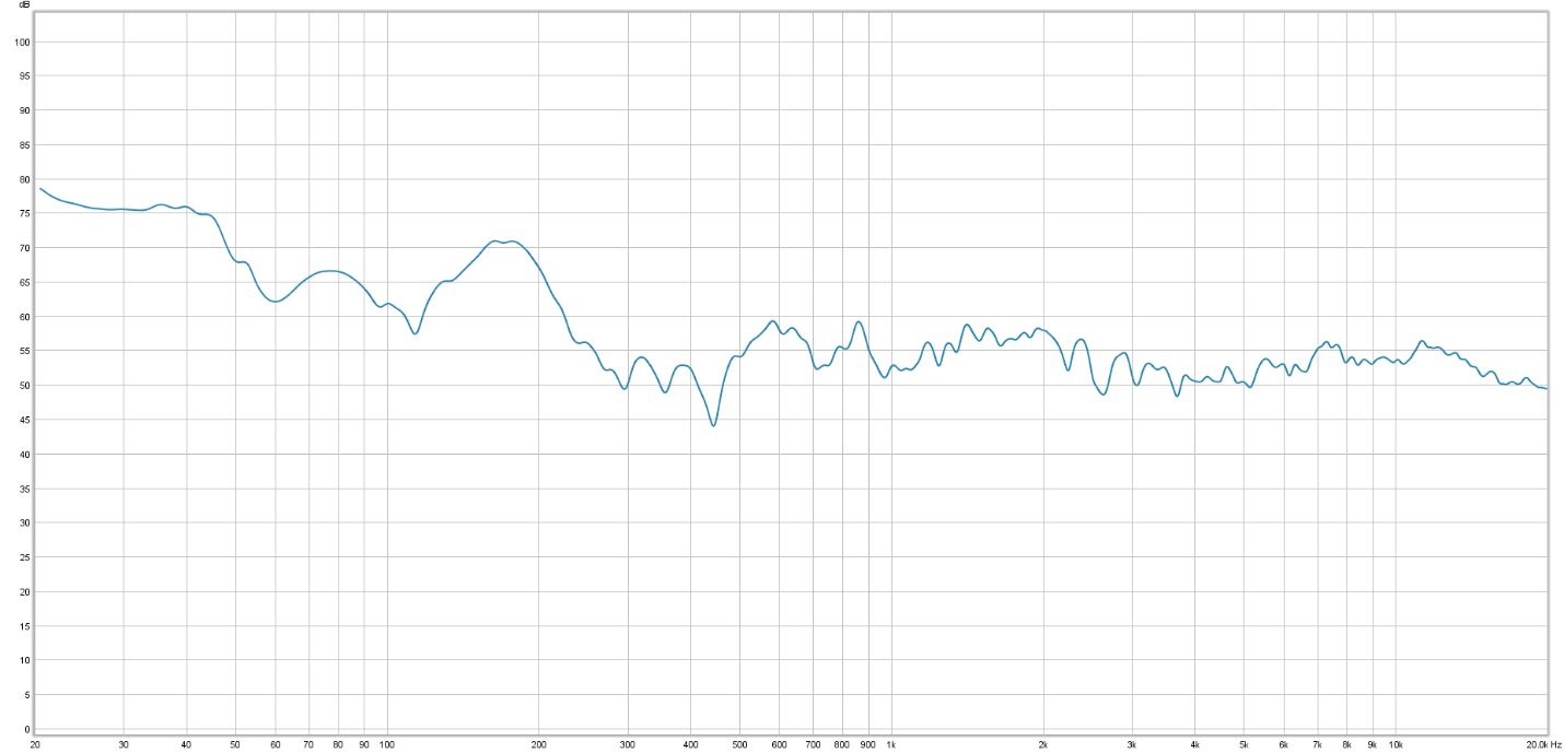
Figure three is a graph that shows the average of the five measurements along with one of those original five. Besides the really narrow peaks and dips, the overall shapes are pretty similar.
Figure 3.
[Figure 3 Caption: Average measurement and one of the original 5 measurements. No smoothing.]

What if we smooth the single mic measurement? Will it look more similar to the average? Figure 4 shows the average of the five measurements and our single mic measurement smoothed to 1/12 octave. With a few small exceptions, they match pretty well.
Figure 4.
[Figure 4 Caption: Unsmoothed average and single mic measurement smoothed to 1/12 octave.]
Now, if we remember that moving our heads makes small peaks and dips inaudible at frequencies above about 1kHz, maybe at frequencies above 1kHz, further smoothing will provide better correlation.
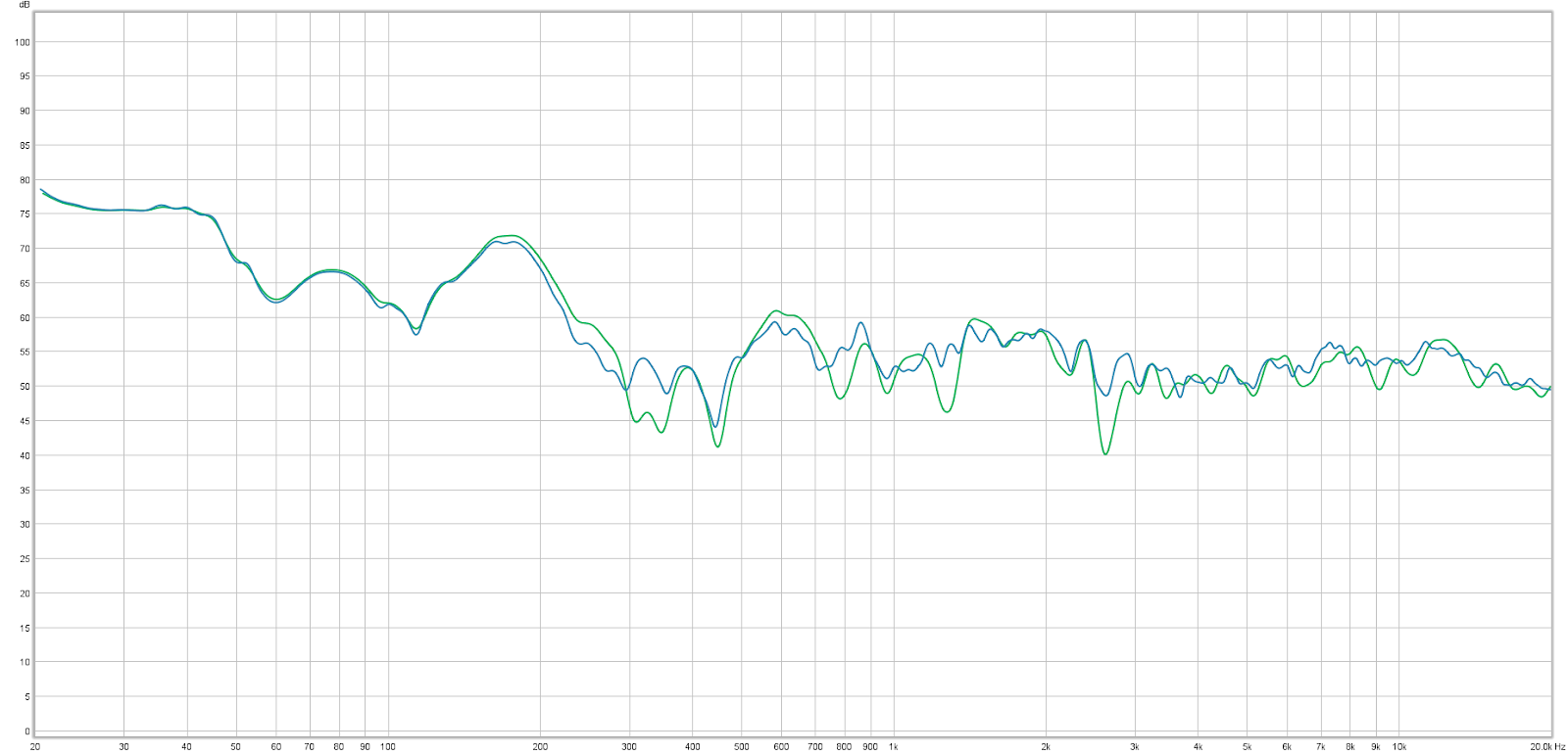
In figure 5, I’ve applied 1/6 octave smoothing to both the average and the single mic measurement and they correlate much better. There are a few small exceptions at 2.6kHz, 1.2kHz, 602Hz, 445Hz and 334Hz. Everywhere else the curves match pretty well. So a single mic measurement smoothed to 1/6 octave, might almost be a suitable substitute for a spatial average if it weren’t for those five frequencies.
Figure 5.

[Figure 5 Caption: Both measurements smoothed to 1/6th octave.]
If we look more carefully we’ll see that at every one of those points where the single mic measurement differs from the average, the peak or the dip in the single mic measurement is narrow. We shouldn’t equalize those. If we’re using a parametric EQ in our process, then we can make a simple rule that we shouldn’t use a filter with a Q value higher than 6. That simple rule will prevent us from equalizing what shouldn’t be equalized.
So, what have we discovered? In a basic sense, we’ve determined that a single mic measurement with 1/6 octave smoothing is sufficient to approximate a spatial average around the listener’s head. We’ve also determined that we should limit our parametric EQ filters to Q values lower than 6. That’s simple. Now we can analyze in real time while we make our adjustments and also see the results in real time. We’ve also applied a limit to our equalization process that prevents us from getting lost in the weeds. We’ve optimized our process for speed, cost and appropriate accuracy, based on what’s audible. We’ve built ourselves a basic algorithm that improves efficiency while maintaining the accuracy that’s necessary.